Chap 3: Image Grayscale Transform⚓︎
约 2773 个字 预计阅读时间 14 分钟
核心知识
- 灰度感知:韦伯定律、可视阈值
- 图像可视度增强:对数化操作
- 图像直方图:灰度图、彩色图、特征
- 直方图均衡化:连续型、离散型(理解具体步骤)
- 直方图匹配
- 直方图变换:线性、非线性

Visibility of Images⚓︎
Grayscale Perception⚓︎
灰度级感知:有 32 灰度级、64 灰度级、128 灰度级、256 灰度级。

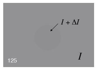
下图给出了一个灰色的矩形,里面有一个颜色略深一点的圆圈(如果你看得见的话
韦伯定律(Weber's Law) 给出了可视阈值的公式:
假设连续两个灰度级之间的亮度差异就是韦伯定律中的可视阈值,那么
根据实际经验知,\(K_{Weber} \in [0.01, 0.02]\),\(\dfrac{I_{\text{max}}}{I_{\text{min}}} = [13, 156]\)。因此,传统的电子设备的显示对比度 (display contrast) 为:
- 阴极射线管:100:1
- 纸上打印:10:1
费希纳定律 (Fechner's Law):人的感知能力是服从 \(\log(I)\) 的。
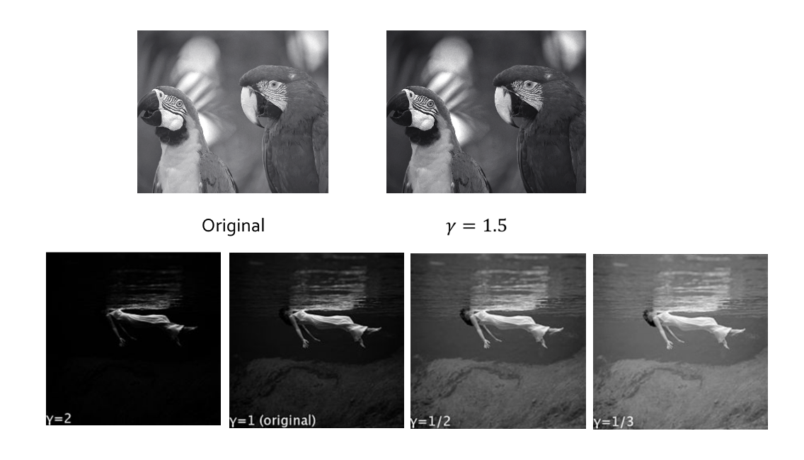
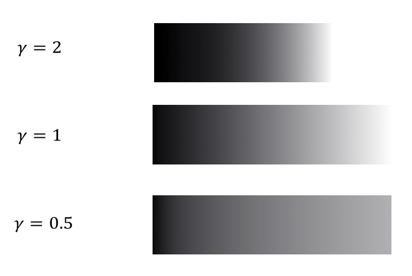
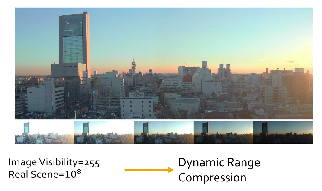
\(\gamma\) Correction⚓︎
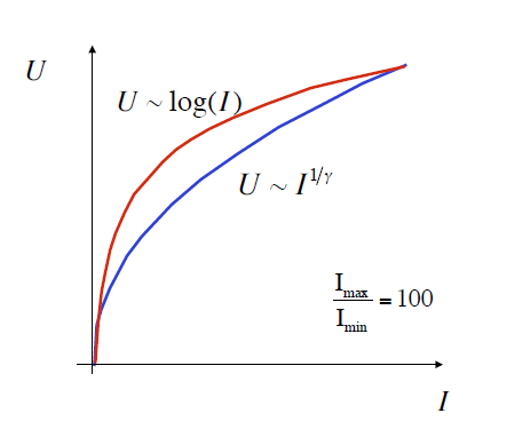
\(\gamma\) 校正:在阴极射线管的显示中,通过调整电压来影响其亮度和变化曲率,从而影响可视性和对细节的表现能力,即 \(U \sim I^{\frac{1}{\gamma}}\),对应曲线图如下(理想情况下,该公式对应的曲线接近于 \(\log(I)\)
例子
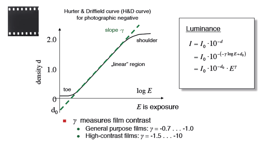
\(\gamma\) 校正在照相技术中的应用:
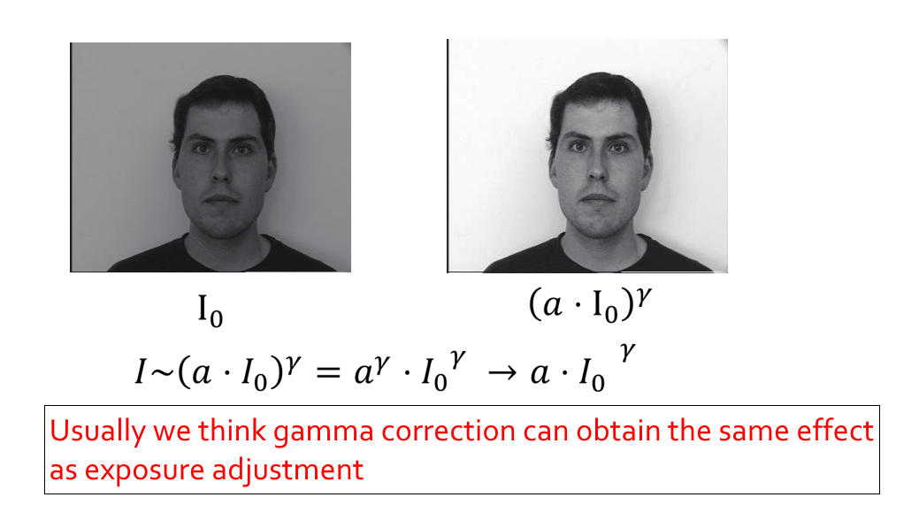
对图像进行 \(\gamma\) 校正:
Visibility Enhancement: a Logarithmic Operation⚓︎
可视能力与高动态范围图像:
为了增强图像的可视性,我们需要对图像中的像素进行基于对数的操作:
其中 \(L_d\) 表示显示亮度,\(L_w\) 表示真实世界的亮度(原图的亮度
注意
用上述公式计算出来的亮度 \(L_d\) 取值范围为 \([0, 1]\),所以要转化为灰度图或彩色图时需要再乘上 255
效果
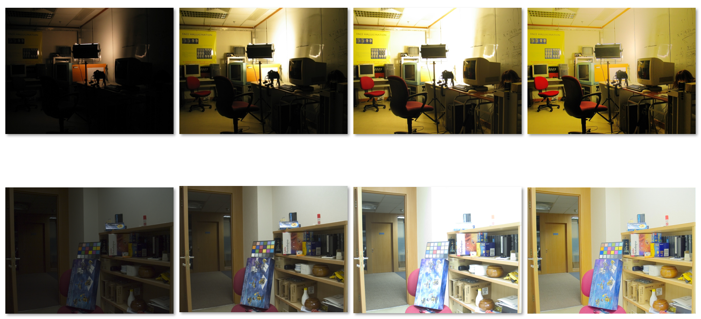
Image Histogram⚓︎
Grayscale Images⚓︎
灰度图的基本概念:
- 灰度图是一个由像素构成的,大小为 \(M \times N\) 的二维数组
- 每个像素用 8 位表示,灰度被分为 \(2^8 = 256\) 个等级,灰度强度 \(p \in [0, 255]\)
- 灰度强度更小,像素越黑
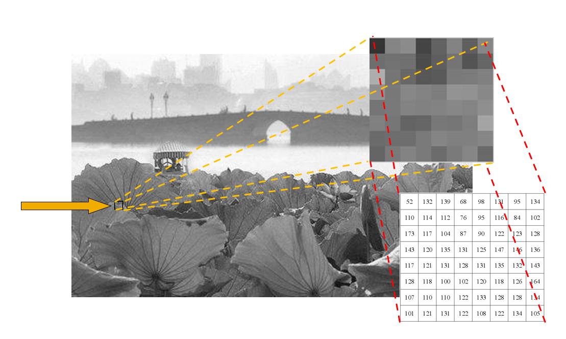
灰度直方图(grayscale histogram):一类统计图形,它表示一幅图像中各个灰度等级的像素个数在像素总数中所占的比重。
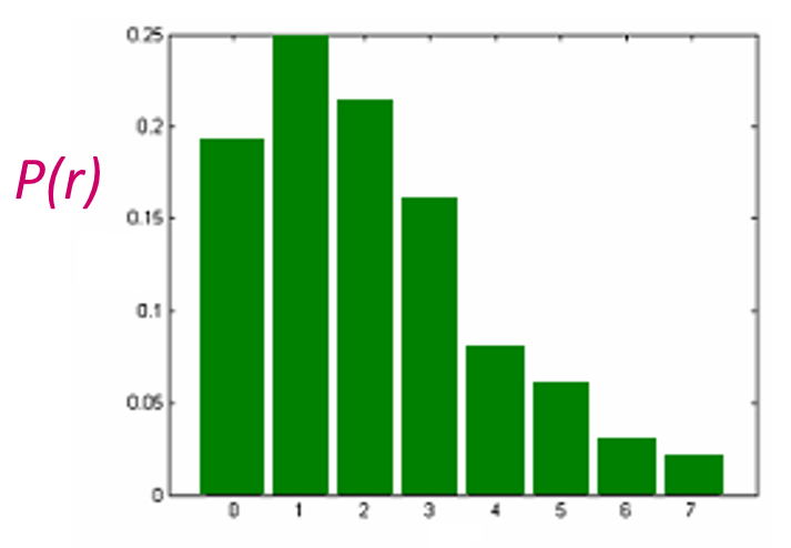
- 纵坐标表示各个灰度等级的像素个数在像素总数中所占的比重
- 横坐标表示灰度等级
设灰度等级范围为 \([0, L-1]\) ,灰度直方图用下列离散函数来表示:
其中,\(r_k\) 为第 \(k\) 级灰度,\(n_k\) 是图像中具有灰度级 \(r_k\) 的像素数目,\(n\) 为图像总像素数,\(0 \le k \le L - 1, 0 \le n_k \le n - 1\)。
通常用概率密度函数来归一化直方图:\(P(r_k) = \dfrac{n_k}{n}\) \(P(r_k)\)为灰度级\(r_k\)所发生的概率(概率密度函数),此时满足下列条件:\(\sum\limits_{k = 0}^{L - 1}P(r_k) = 1\)
例子
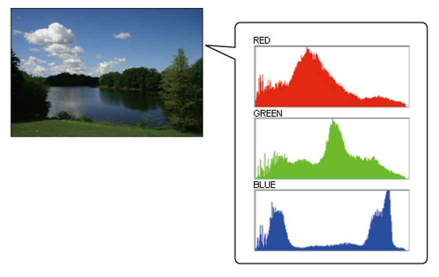
Color Images⚓︎
彩色直方图(color histogram):一类统计图形,它表示一幅图像中 r, g, b 通道上各个灰度等级的像素个数在像素总数中所占的比重。
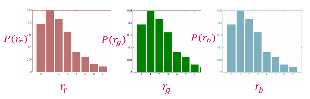
例子
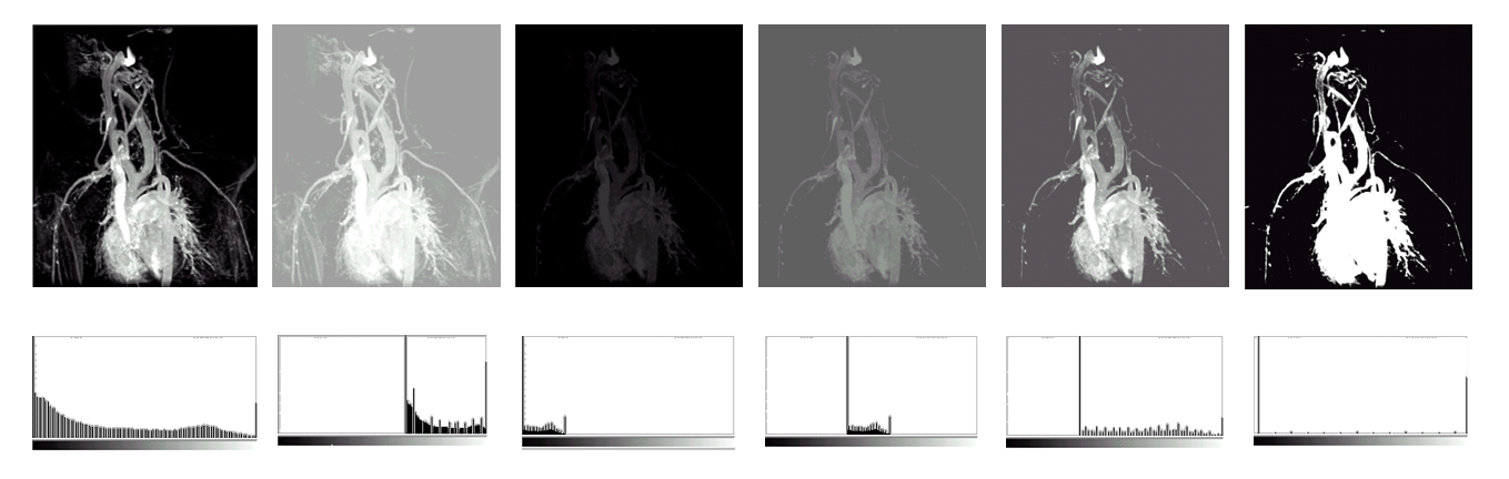
Characteristics of histogram⚓︎
直方图的特征:
- 是空间域处理技术的基础
- 反映图像灰度的分布规律,但不能体现图像中的细节变化情况
- 对于一幅给定的图像,其直方图是唯一的
-
不同的图像可以对应相同的直方图,比如下面这三张图的灰度直方图是一样的
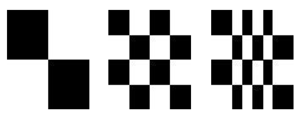
-
直方图被有效地用于图像增强、压缩和分割 , 是图像处理的一个实用手段。
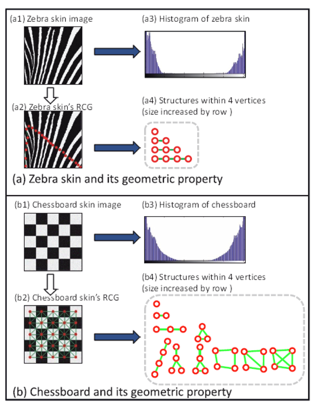
直方图的缺点:
- 带来噪声
- 丢失结构信息:只知颜色分布,不知结构
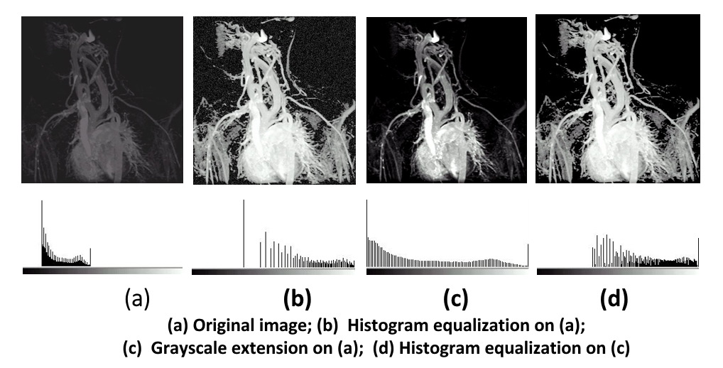
例子
Histogram Equalization⚓︎
直方图均衡化(historam equalization):将原图像的非均匀分布的直方图通过变换函数 \(T\) 修正为均匀分布的直方图,然后按均衡直方图修正原图像。图像均衡化处理后,图像的直方图是平直的,即各灰度级具有相同的出现频数。
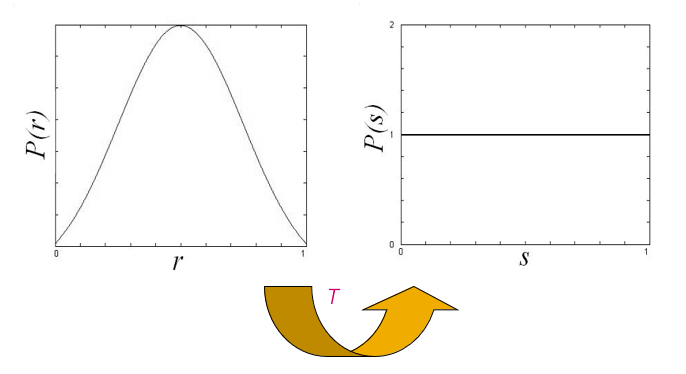
直方图均衡化的关键在于找到变换函数 \(T\)。在计算前,我们做出以下假设和规定:
- 假设:
- 令 \(r\) 和 \(s\) 分别代表变化前后图像的灰度级,并且 \(0 \le r,s \le 1\)
- \(P(r)\) 和 \(P(s)\) 分别为变化前后各级灰度的概率密度函数(\(r\) 和 \(s\) 值已归一化,最大灰度值为 1)
- 规定:
- \(T(r)\) 是单调递增函数,并且 \(0 \le r \le 1\),\(0 \le T(r) \le 1\)
- 反变换 \(r = T^{-1}(s)\) 也为单调递增函数
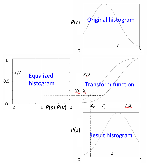
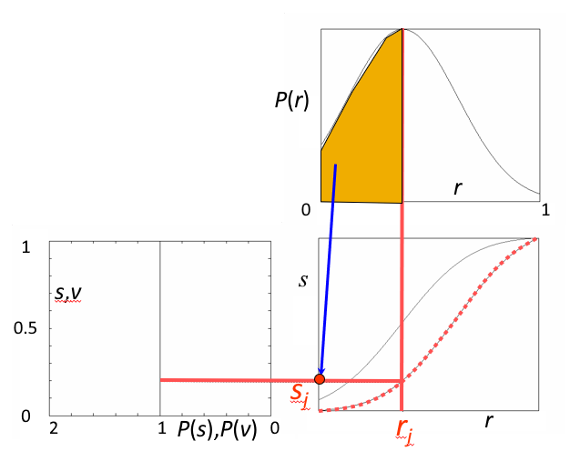
Continuous Version⚓︎
考虑到灰度变换不影响像素的位置分布,也不会增减像素数目。所以有:
几何意义:转换函数 \(T\) 在变量 \(r\) 处的函数值 \(s\),是原直方图中灰度等级为 \([0, r]\) 以内的直方图曲线所覆盖的面积。
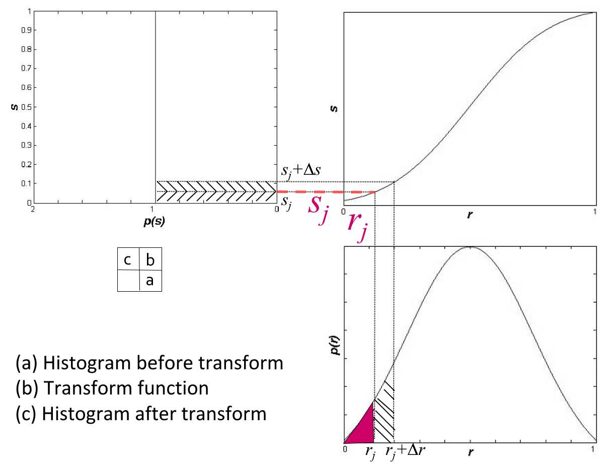
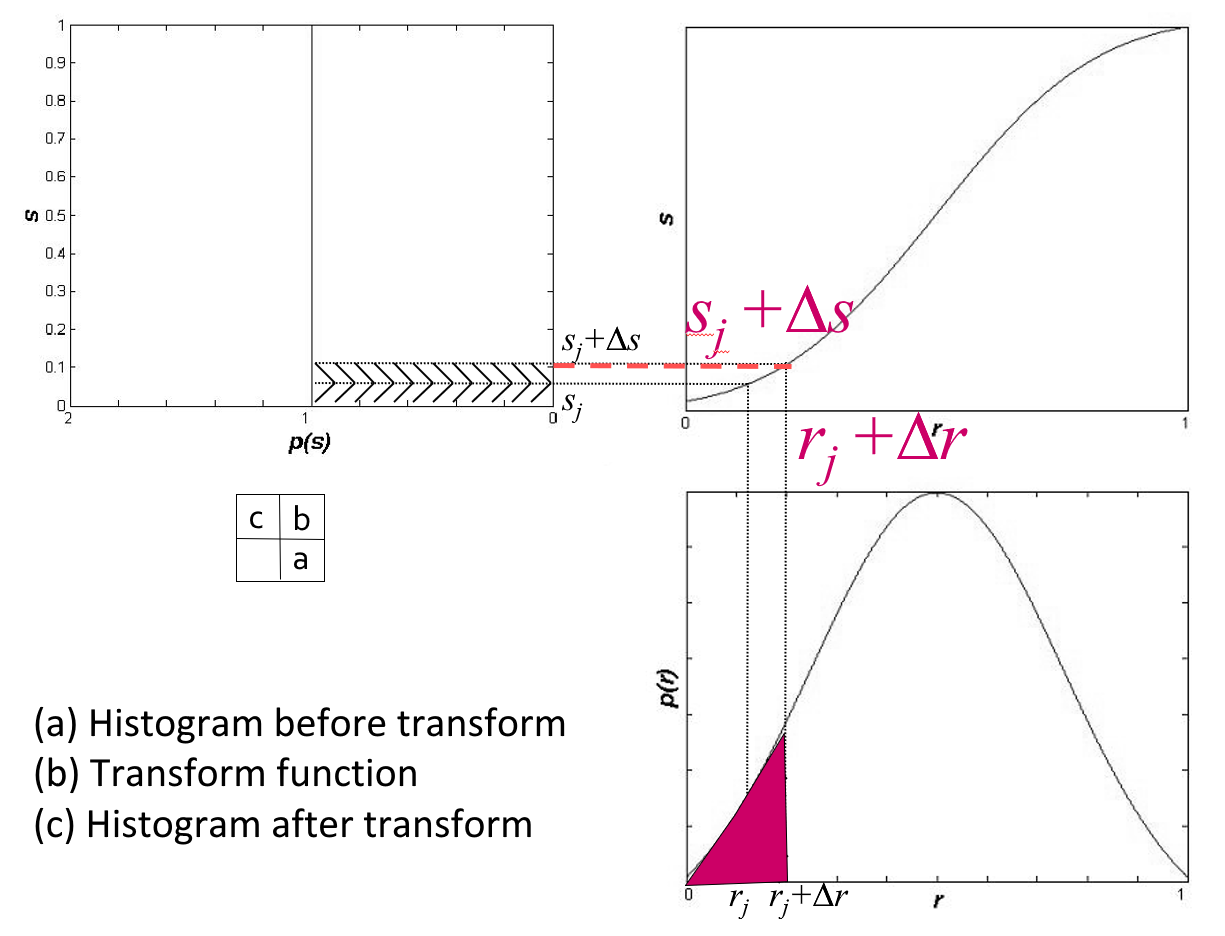
其中右下为原来的直方图,右上为变换函数,左上为均衡化后的直方图。
Discrete Version⚓︎
设一幅图像的像素总数为 \(n\),分 \(L\) 个灰度级,\(n_k\) 为第 \(k\) 个灰度级出现的像素数,则第 \(k\) 个灰度级出现的概率为:
离散灰度直方图均衡化的转换公式为:
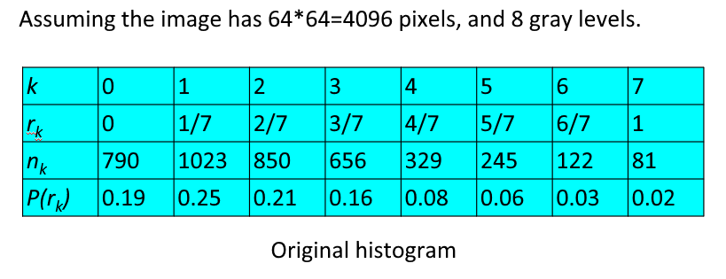
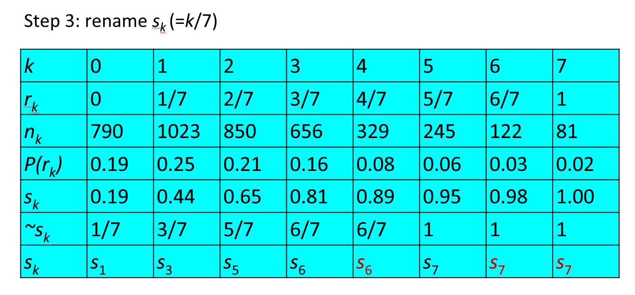
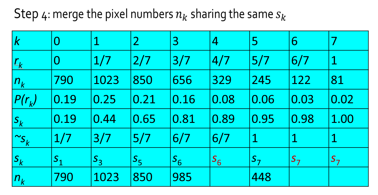
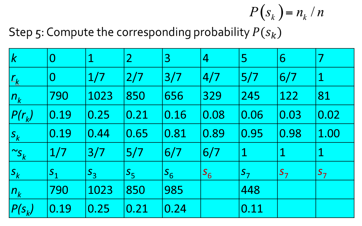
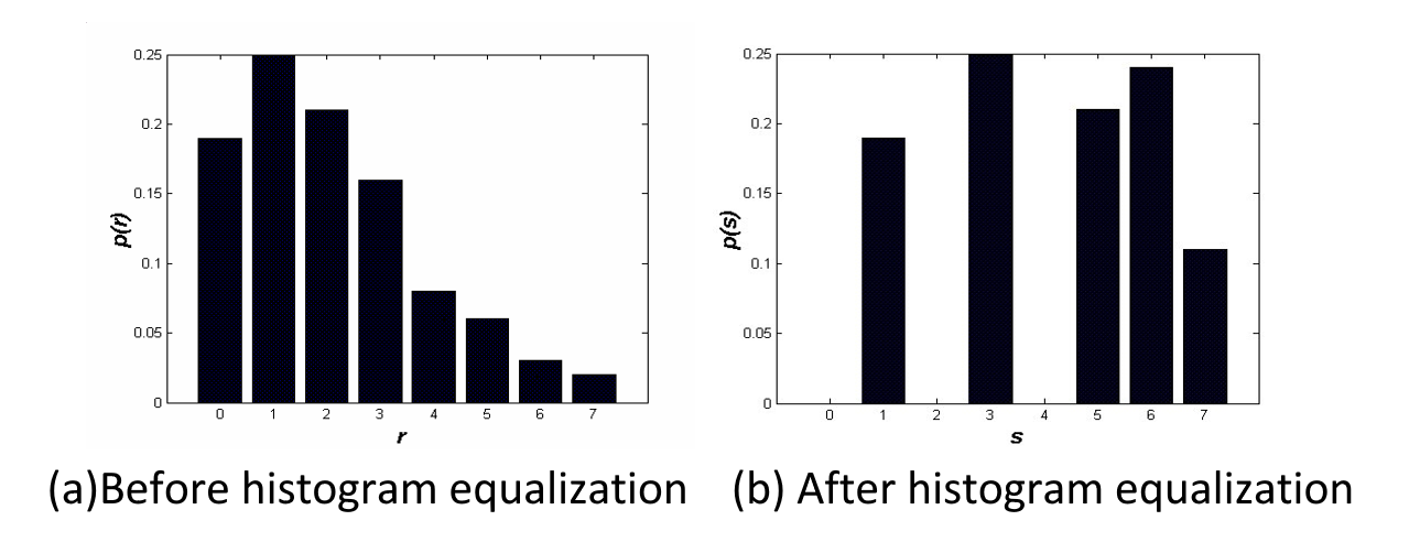
例子
这是原来直方图的数据,请对它进行均衡化操作。
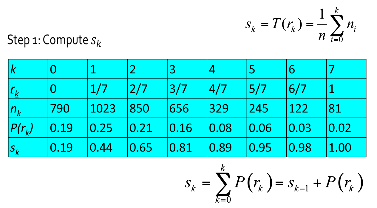
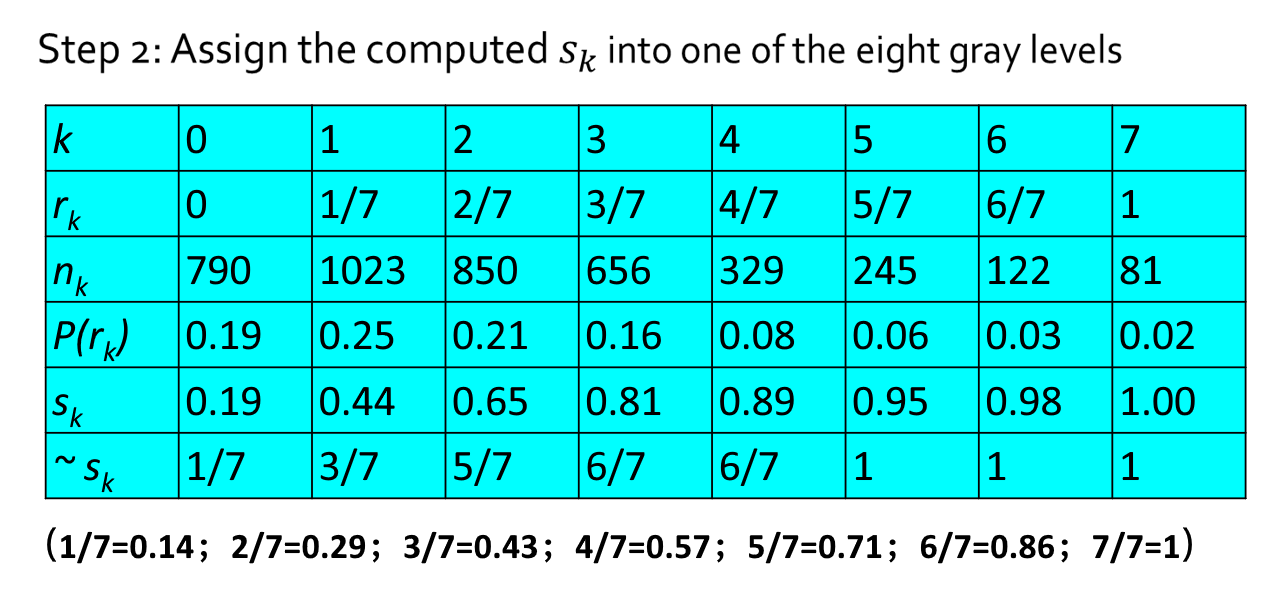
注意:我们对 \(s_k\) 进行了重命名操作,\(k\) 要从 1 开始数了
思考
按照均衡化的要求,在均衡化后的结果直方图中,各灰度级发生的概率应该是相同的或大致接近的,但结果是右下图中离散灰度级均衡化后,各灰度级出现的概率并不完全一样,这是为什么呢?
答案
步骤 2 中,所得的 \(s_k\) 不可能正好等于 8 级灰度值中的某一级,因此需要就近归入某一个灰度级中。这样,相邻的多个 \(s_k\) 就可能落入同一个灰度级,需要在步骤 3 时将处于同一个灰度级的像素个数累加。因此,离散灰度直方图均衡化操作以后,每个灰度级处的概率密度(或像素个数)并不完全一样。
总结
- 记忆方法:直方图均衡化 \(\approx\) 概率密度函数 -> 概率分布函数
- 直方图均衡化实质上是减少图像的灰度级以换取对比度的加大。在均衡过程中,原来的直方图上出现概率较小的灰度级被归入很少几个甚至一个灰度级中,故得不到增强。若这些灰度级所构成的图像细节比较重要,则需采用局部区域直方图均衡化处理。
Histogram Fitting⚓︎
直方图匹配(histogram fitting):修改一幅图像的直方图,使得它与另一幅直方图匹配。直方图匹配的目标,是突出我们感兴趣的灰度范围,使图像质量改善。利用直方图均衡化操作,可以实现直方图匹配过程。

Continuous Version⚓︎
操作步骤
根据第一个变换函数
将原始直方图的 \(r\) 映射到 \(s\) 上。
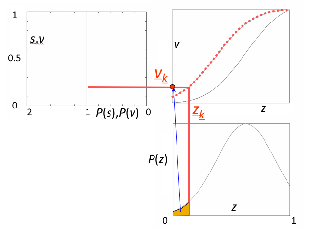
根据第二个变换函数
将结果直方图的 \(z\) 映射到 \(v\) 上。
由 \(v = G(z)\) 得到 \(z =G^{-1}(v)\)。由于 \(s\) 和 \(v\) 有相同的分布,逐一取 \(v = s\),求出与 \(r\) 对应的 \(z =G^{-1}(s)\)。
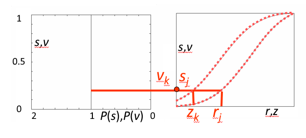
Discrete Version⚓︎
- 在步骤 1 和 2 中,分别计算获得两张表(参见直方图均衡化中的算例)
- 从中选取一对 \(v_k\)、\(s_j\),使 \(v_k = s_j\)
- 从两张表中查出对应的 \(z_k\)、\(r_j\)
- 这样,原始图像中灰度级为 \(r_j\) 的所有像素都映射成灰度级 \(z_k\),最终得到所期望的图像
Histogram Transform⚓︎
直方图变换(histogram transform):用以确定变换前后两个直方图灰度级之间对应关系的变换函数。经过直方图变换以后,原图像中的任何一个灰度值都唯一对应一个新的灰度值,从而构成一幅新图像。前面讲过的直方图均衡化、直方图匹配都属于直方图变换操作。
应用:图像增强
- 采用一系列技术去改善图像的视觉效果,或将图像转换成一种更适合于人或机器进行分析处理的形式。
- 图像增强并不以图像保真为准则,而是有选择地突出某些对人或机器分析有意义的信息,抑制无用信息,提高图像的使用价值。
- 根据任务目标突出图像中感兴趣的信息,消除干扰,改善图像的视觉效果或增强便于机器识别的信息。
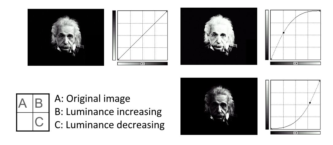
例子
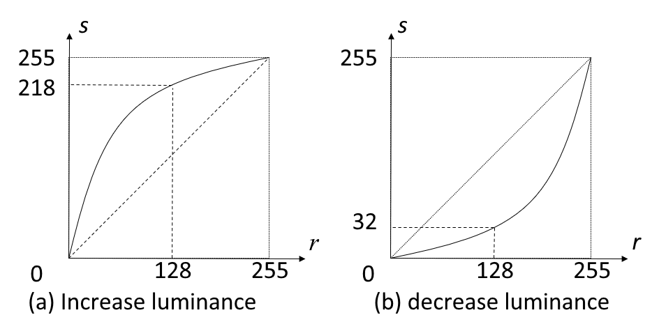
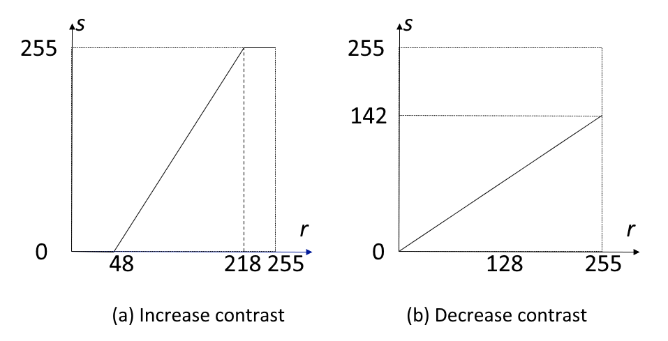
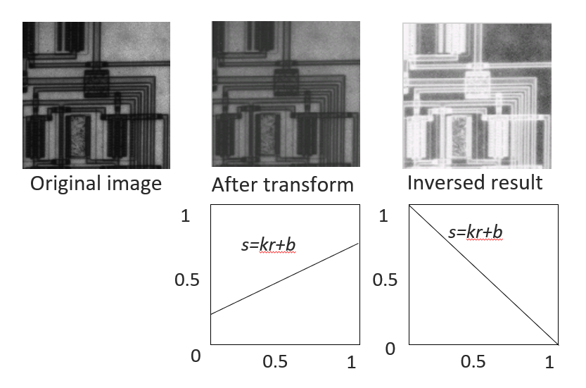
Linear Transform⚓︎
一般的线性变换函数及其图像如下所示:
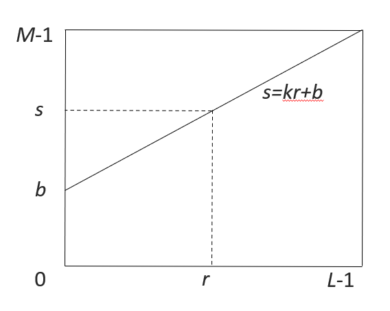
其中,\(r\) 为输入点的灰度值,\(s\) 为相应输出点的灰度值,\(k\)、\(b\) 为常数。
例子
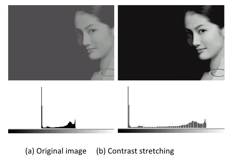
应用
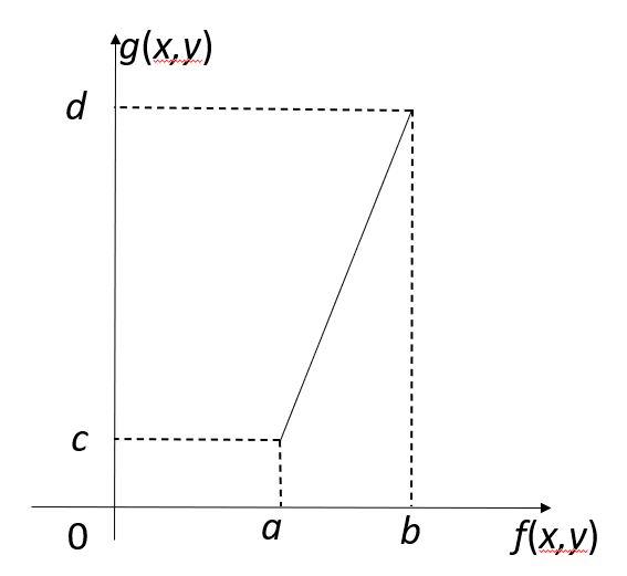
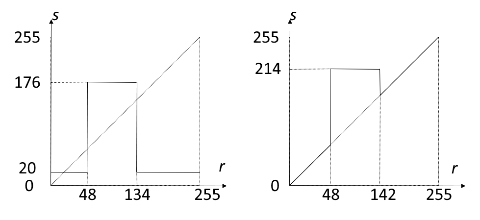
其中,输入图像 \(f(x, y)\) 灰度范围为 \([a, b]\),输出图像 \(g(x, y)\) 灰度范围为 \([c, d]\)。
例子
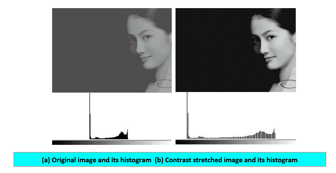
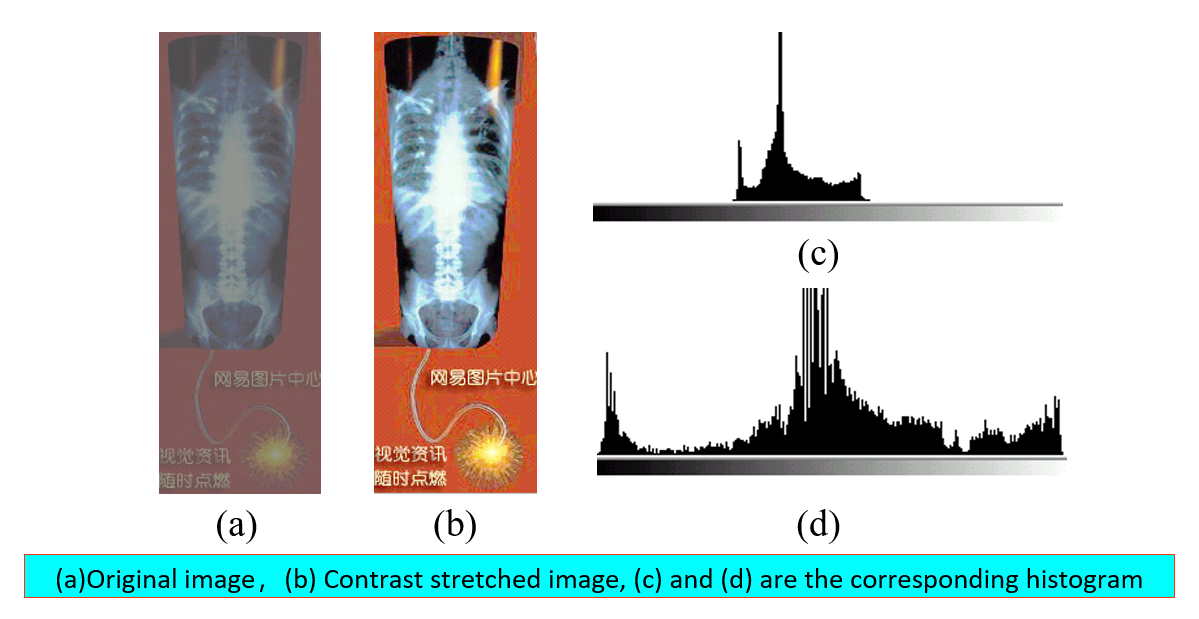
利用分段直方图变换,可以将感兴趣的灰度范围线性扩展,同时相对抑制不感兴趣的灰度区域。
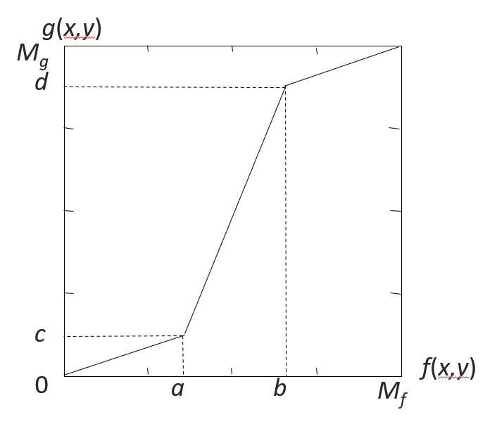
其中 \(f(x, y) \in [0, M_f], g(x, y) \in [0, M_g]\)。
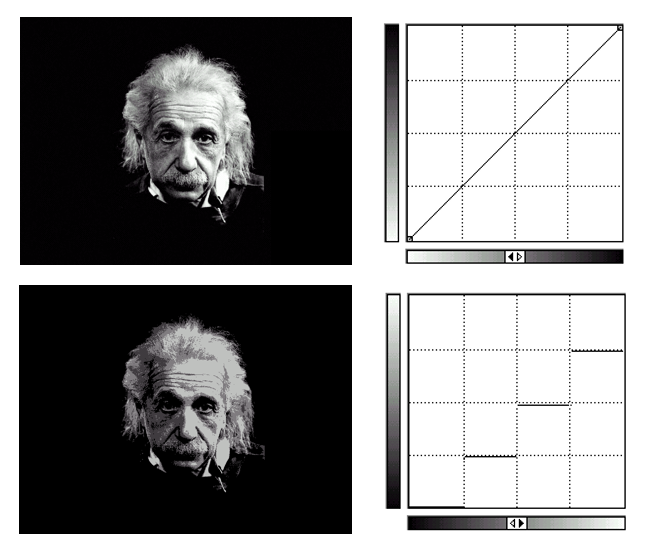
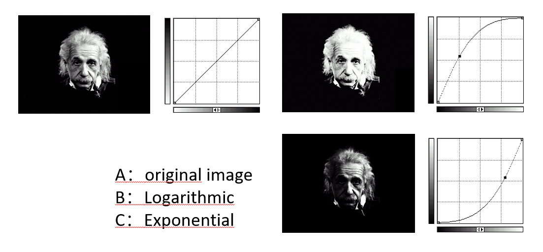
Nonlinear Transform⚓︎
对数函数和指数函数是常见的非线性变换函数。
-
对数变换 (logarithmic transform)
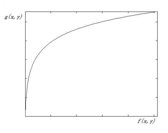 \[ g(x, y) = a + \dfrac{\ln[f(x, y) + 1]}{b \ln c} \]
其中 \(a, b, c\) 是可调节的。
-
指数变换 (exponential transform)
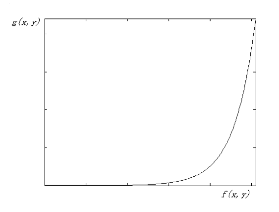 \[ g(x, y) = b^{c[f(x, y) - a]} - 1 \]
其中 \(a, b, c\) 是可调节的。
例子
评论区