Chap 5: Hashing⚓︎
约 2199 个字 210 行代码 预计阅读时间 14 分钟
核心知识
- 散列函数
- 单独链表法
- 开放地址
- 线性探测
- 二次探测
- 双重散列法
- 再散列
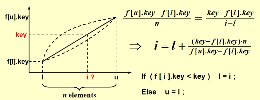
引入:插值排序 (interpolation sort)
在 Chap 7 中,我们介绍了一些基于比较的排序算法,这类算法的最优时间复杂度为 \(O(n \log n)\),然而这不是排序算法的极限——插值排序为我们提供了时间复杂度仅为 \(O(1)\) 的方法,其本质为基于公式的搜索 (search by formula)。
题目:从有序列表 f[l].key, f[l+1].key, ..., f[u].key 中找到特定的 key
General Idea⚓︎
简单表 (symbol table) ADT
-
Objects:一组 " 名称 + 属性 " 对的集合,集合中的每个名称是唯一的
-
Operations:
SymTab Create(TableSize)Boolean IsIn(symtab, name)Attribute Find(symtab, name)
SymTab Insert(symtab, name, attr)SymTab Delete(symtab, name)
散列表 (hash tables)
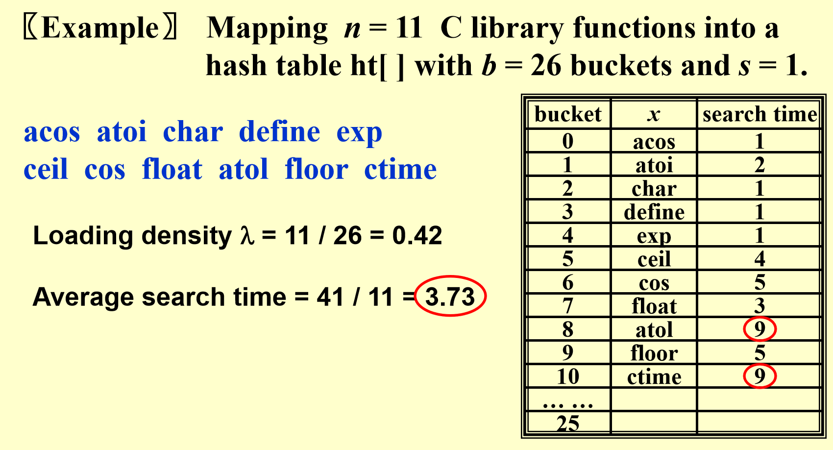
对于每个标识符 x,我们定义一个散列函数 (hash function) f(x),用来表示 x 在 ht[] 的位置,即下图中包含 x 的篮子 (bucket) 的索引
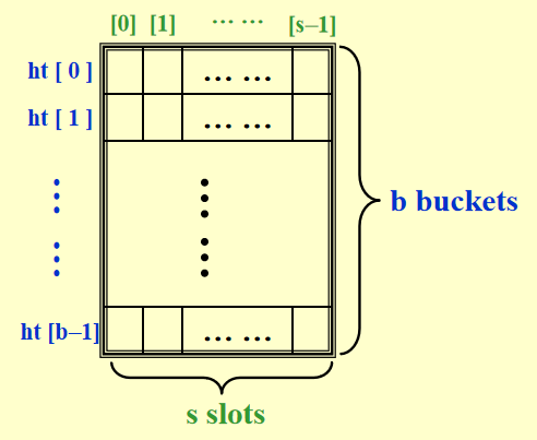
- T 表示标识符的总数
- n 表示 ht[] 中(即已排好序的)标识符的总数
- 标识符密度 (identifier density) = \(\dfrac{n}{T}\)
- 加载密度 (loading density)\(\lambda = \dfrac{n}{s \cdot b}\)
散列表的常见问题
- 冲突 (collision):2 个不同的标识符放入相同的篮子内,即 \(f(i_1) = f(i_2)\) 且 \(i_1 \ne i_2\)
- 溢出 (overflow):某个(些)篮子的空间已满,无法安置新的标识符
注:当篮子容量 s = 1 时,冲突和溢出同时发生
Example
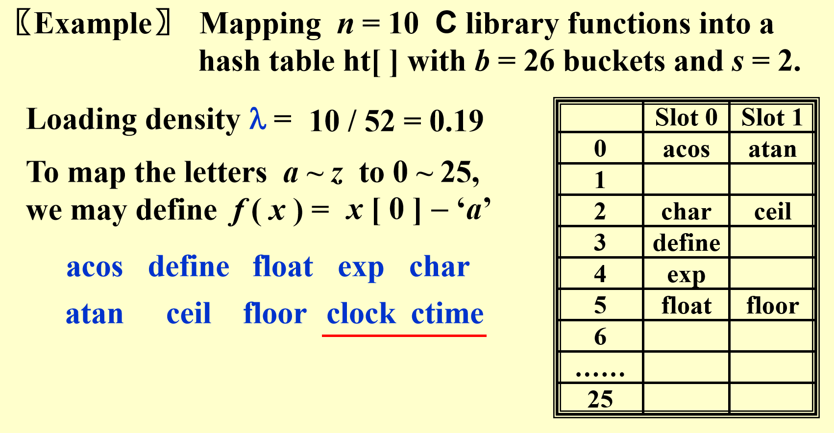
若没有溢出,散列表的主要操作的时间复杂度均为常数级,即:
Hash Function⚓︎
散列函数 f 的性质:
- f(x) 必须容易计算,且能最小化冲突的可能
- f(x) 不能有 " 偏见 ",能够将所有的键平均分配至散列表内,也就是说: \(\forall x,\ \forall i\),\(f(x) = i\) 的概率为 \(\dfrac{1}{b}\)。这样的散列函数被称为统一散列函数 (uniform hash function)
一些散列函数
x 为整数
这不是一个好的散列函数,因为用这种函数很容易发生冲突。然而,若我们让 \(TableSize\) 为一个质数,且令所有的键尽可能随机,冲突就不那么容易发生了
x 为字符串
这是前一种函数的变种,用于字符串的情况,\(\sum x[i]\) 为所有字符的 ASCII 码之和。这种方法也很简单,也很容易产生冲突
x 为长度为 3 的英文字符串(全大写或全小写
) (27 = 26 个字母 + NULL( 空 ))
这是对前一种函数的改良,把每个字符串表示为一个唯一的 27 进制数。这确实能完全避开冲突,然而实际长度为 3 的英语单词的个数远少于散列表的篮子个数,从而导致空间的巨大浪费
如果我们将 27 改成 32,则用左移 5 位的运算替代乘以 26 的运算,效率更高 ( 移位的速度大于乘法 )。由于是左移位,所以需要稍微调整一下散列值的表示,如下图所示
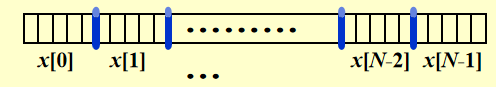
代码:
缺点:若字符串 x 太长,那么最先进入散列值的字符会被左移到边界外面,因此我们需要谨慎挑选 x 的字符Separate Chaining⚓︎
单独链表法 (separate chaining):将所有散列值相同的键放入同一张链表中
注:这种方法又被称为开散列法 (open hashing)
代码实现
- 初始化
struct ListNode;
typedef struct ListNode * Position;
struct HashTbl;
typedef struct HashTbl * HashTable;

struct ListNode
{
    ElementType Element;
    Position Next;
};
typedef Position List;

/* List *TheList will be an array of lists, allocated later */
/* The lists use headers (for simplicity), */
/* though this wastes space */
struct HashTbl
{
    int TableSize;
    List * TheLists;
};
- 创建空表
HashTable InitializeTable(int TableSize)
{
    HashTable H;
    int i;
    if (TableSize < MinTableSize)
    {
        Error("Table size too small");
        return NULL;
    }
    H = (HashTable)malloc(sizeof(struct HashTbl)); // Allocate table
    if (H == NULL)
        FatalError("Out of Space!!!");
    H->TableSize = NextPrime(TableSize);  // Better be prime
    H->TheLists = malloc(sizeof(List) * H->TableSize);  // Array of lists
    if (H->TheLists == NULL)
        FatalError("Out of space!!!");
    for(i = 0; i < H->TableSize; i++)
    {   // Allocate list headers
        H->TheLists[i] = malloc(sizeof(struct ListNode)); // Slow!
        if ( H->TheLists[i] == NULL )
            FatalError("Out of space!!!");
        else
            H->TheLists[i]->Next = NULL;
    }
    return H;
}
散列表示意图
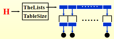
注意:散列表的开头,以及每个篮子都是有 " 空头 " 的,这主要是为了删除操作的方便。若没有删除操作,则最好不要用空头,这样可以节省空间
- 从散列表中找键
Position Find(ElementType Key, HashTable H)
{
    Position P;
    List L;

    L = H->TheLists[Hash(Key, H->TableSize)];

    P = L->Next;
    // Identical to the code to perform a Find for List ADT
    while (P != NULL && P->Element != Key) // Probably need strcmp
        P = P->Next;
    return P;
}
- 将键插入散列表内(放在篮子的最上(前)面)
void Insert(ElementType Key, HashTable H)
{
    Position Pos, NewWell;
    List L;
    Pos = Find(Key, H);
    if (Pos == NULL) // Key is not found, then insert
    {
        NewCell = (Position)malloc(sizeof(struct ListNode));
        if (NewCell == NULL)
            FatalError("Out of space!!!");
        else
        {
            L = H->TheLists[Hash(Key, H->TableSize)];
            NewCell->Next = L->Next;
            NewCell->Element = Key; // Probably need strcpy
            L->Next = NewCell;
        }
    }
}
注:
- 不好的一点是该函数用了两次
Hash()函数,所以这里需要改进一下- 我们要让
TableSize尽可能接近键的数量,即让加载密度 \(\lambda \approx 1\)- 这里仅考虑所有键都不同的情况,若出现相同的键,要么选择无视,要么增加一个额外的字段记录重复的次数
Open Addressing⚓︎
开放地址 (open addressing):通过寻找下一个空的单元来解决冲突,这样我们就不必使用指针了。
注:这种方法又被称为闭散列法 (close hashing)
模版:
Algorithm: insert key into an array of hash table
{
    index = hash(key);
    initialize i = 0  // the counter of probing
    while (collision at index)
    {
        index = (hash(key) + f(i)) % TableSize;
        if (table is full) break;
        else i++;
    }
    if (table is full)
        ERROR("No space left");
    else
        Insert key at index;
}
正如 while 循环所示,若使用一次冲突解决函数后,冲突仍然发生,那就继续使用冲突解决函数,直至冲突解决,或发现无法解决直接退出。
Linear Probing⚓︎
最简单的冲突解决函数为线性探测 (linear probing):f(i) = i,它仅是一个线性函数
线性探测中预期探测次数关于加载密度的表达式:
对于上面的例子,p = 1.36。虽然很小,但是在最坏情况下 p 会很大。
线性探测的问题:基本聚集 (primary cluster)
线性探测将位置不匹配的键安放至后面最近的空内,这样做会形成区块 (cluster),使得散列表分布不均匀,导致即使表的空间看起来挺空的,但是某些地方聚集了一堆元素。
随机冲突解决策略 (random collision resolution strategy)
- 不成功的探测次数:\(\dfrac{1}{1 - \lambda}\)
- 成功探测的平均次数 = 不成功的探测次数
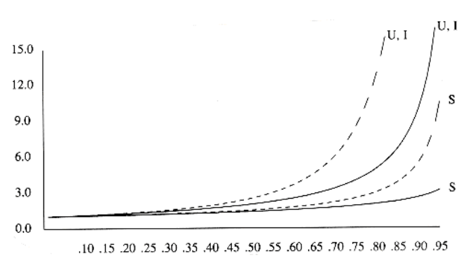
线性探测与随机策略的效率比较(其中 S 表示成功的搜索,U 表示不成功的搜索,I 表示插入)
Quadratic Probing⚓︎
二次探测 (quadratic probing) 的函数为:\(f(i) = i^2\)
定理:若使用二次探测,且表的大小是一个质数,则当表至少有一半的空余空间时,新的元素总是能够被成功插入。
证明
只要证明前 \(\lfloor \dfrac{TableSize}{2} \rfloor\) 个可替代的位置是不同的,也就是说,\(\forall\ 0 < i \ne j \le \lfloor \dfrac{TableSize}{2} \rfloor\),我们有:
反证法:假设 \(h(x) + i^2 \equiv h(x) + j^2 (\text{mod }\ TableSize)\),那么可以得到 \((i + j)(i - j) \equiv 0(\text{mod } TableSize)\),即 (i + j) 或 (i - j) 能够被质数 TableSize 整除,但这显然是不可能的,推出矛盾,因此定理成立。
注
若表的大小是一个形如 4k + 3 的质数,则使用二次探测 \(f(i) = \pm i^2\) 来探测整张表
代码实现
- 声明
#ifndef _HashQuad_H

typedef unsigned int Index;
typedef Index Position;

struct HashTbl;
typedef struct HashTbl *HashTable;

HashTable InitializeTable(int TableSize);
void DestroyTable(HashTable H);
Position Find(ElementType Key, HashTable H);
void Insert(ElementType Key, HashTable H);
ElementType Retrieve(Position P, HashTable H);
HashTable Rehash(HashTable H);
// Routine such as Delete and MakeEmpty are omitted

#endif // _HashQuad_H

// Place in the implementation file

enum KindOfEntry {Legitimate, Empty, Deleted};

struct HashEntry
{
    ElementType Element;
    enum KindOfEntry Info;
};

typedef struct HashEntry Cell;

// Cell * TheCells will be an array of HashEntry cells, allocated later
struct HashTbl
{
    int TableSize;
    Cell * TheCells;
};
- 初始化
HashTable InitializeTable(int TableSize)
{
    HashTable H;
    int i;

    if (TableSize < MinTableSize)
    {
        Error("Table size too small");
        return NULL;
    }

    // Allocate table
    H = (HashTable)malloc(sizeof(struct HashTbl));
    if (H == NULL)
        FatalError("Out of Space!!!");

    H->TableSize = NextPrime(TableSize);

    // Allocate array of Cells
    H->TheCells = (Cell *)malloc(sizeof(Cell) * H->TableSize);
    if (H->TheCells == NULL)
        FatalError("Out of Space!!!");

    for (i = 0; i < H->TableSize; i++)
        H->TheCells[i].Info = Empty;

    return H;
}
- 寻找位置
Position Find(ElementType Key, HashTable H)
{
    Position CurrentPos;
    int CollisionNum = 0;
    CurrentPos = Hash(Key, H->TableSize);
    while (H->TheCells[CurrentPos].Info != Empty &&
            H->TheCells[CurrentPos].Element != Key)
    {
        CurrentPos += 2 * ++CollisionNum - 1;  // 1
        if (CurrentPos >= H->TableSize)        // 2
            CurrentPos -= H->TableSize;
    }
    return CurrentPos;  // 3
}
注
若交换 while 循环内的两个判断条件,程序很有可能出现段错误,因为没有先判断是否有元素
- 这里用到二次探测函数的递推关系:\(F(i) = F(i - 1) + 2i - 1\),避免使用乘法,从而提高效率
- 这块语句替换了原来的模除运算,提高了效率;但是若
CurrentPos大于 2 倍的TableSize,就无法实现模除的功能了(因此使用前确保CurrentPos不超过 2 倍的TableSize) - 返回可插入的位置
- 插入元素
注
- 如果有过多的插入和删除操作,插入的效率会显著降低
- 尽管二次探测解决了基本聚集的问题,但它会导致二次聚集:通过散列函数被分配到相同位置的键,探测到相同的可替代的位置。
Double Hashing⚓︎
双散列 (double hashing)的函数:\(f(i) = i * \mathrm{hash}_2(x)\),其中 \(\mathrm{hash}_2(x)\) 为第 2 个散列函数
- \(\mathrm{hash}_2(x) \ne 0\)
- 确保所有位置都能被探测到
较好的散列函数:\(\mathrm{hash}_2(x) = R - (x \% R)\),其中 R 为小于 TableSize 的质数
注
- 若双散列函数能正确执行,那么由模拟结果知,预期的探测次数和随机冲突解决策略的大致相同
- 二次探测不需要使用第二个散列函数,因此在实践中更简单、更快
Rehashing⚓︎
在二次探测中,我们有时会用到“再散列 (rehashing)”的技巧
何时使用再散列
- 被占用的表空间达到一半时
- 插入失败时
- 散列表的加载因数达到特定值时
具体做法:
- 建立一张额外的表,大小是原来的两倍
- 遍历原来的整张散列表中未删除的元素
- 使用新的散列函数,将遍历到的元素插入新的表中
如果表内有 N 个键,则时间复杂度 \(T(N) = O(N)\)
代码实现
HashTable ReHash(HashTable H)
{
    int i, OldSize;
    Cell * OldCells;

    OldCells = H->TheCells;
    OldSize = H->TableSize;

    // Get a new, empty table
    H = InitializeTable(2 * OldSize);

    // Scan through old table, reinserting into new
    for (i = 0; i < OldSize; i++)
        if (OldCells[i].Info == Legitimate)
            Insert(OldCells[i].Element, H);

    free(OldCells);

    return H;
}
评论区